

3D plot – Part 4Different built-in functions to deal with tridimensional graphs.
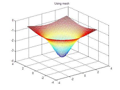
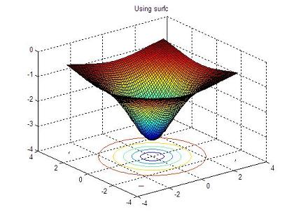
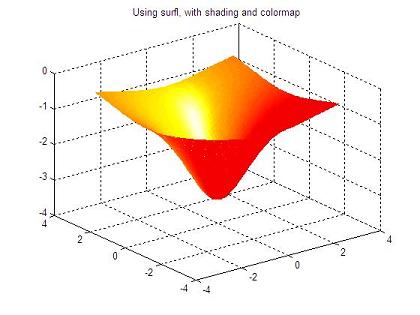
data (a function depending on two variables) using several instructions, so the visualization is pretty different from each other. Example: % cleans the memory workspace clc; clear; close all; % defines the range of axes x and y vx = -3 : 0.1 : 3; vy = vx; % generates the powerful grid [x, y] = meshgrid(vx, vy); % defines the function to be plotted z = -10 ./ (3 + x.^2 + y.^2); % opens figure 1 and plots the function using only contours figure(1) contour3(x,y,z) % opens figure 2 and draws the function using a mesh figure(2) mesh(x,y,z) % opens figure 3 and draws the function using surface with contours figure(3) surfc(x,y,z) % opens figure 4 and draws the function using a enlightened surface figure(4) surfl(x,y,z) shading interp colormap hot The resulting 3D graphics are: 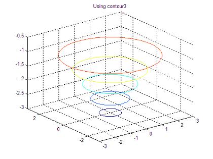
From '3D Plot Part 4' to home From '3D Plot Part 4' to 3D Main
|
undefined
undefined undefined undefined undefined undefined undefined undefined undefined undefined undefined |
undefined
 undefined
 undefined