
Circuit Simulator (WinSpice and Matlab, improved interface)In this
article, an improved Matlab
routine to drive the WinSpice circuit
simulator is
presented. This
method can also be easily adapted to
simulate and drive any circuit entered in SPICE.
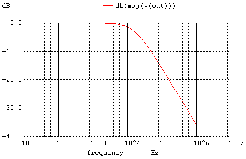
The concept of the Matlab driver is illustrated by simulating a very simple RC low-pass filter. In this example we're using Matlab ver. 7.0.1 and WinSpice3 ver. 1.04.07. A first approach to the circuit driver was presented here. For more information about Matlab, visit www.mathworks.com. For more information about WinSpice, visit www.winspice.com. SPICE stands for Simulation Program with Integrated Circuit Emphasis Interchanging information between Matlab and WinSpice allows the implementation of optimization algorithms and graphical possibilities not included in the circuit simulator environment itself. The approach developed now is very flexible and utilizes the inherent capability of this SPICE simulator to include other circuit text files with parameters, and print data to external .csv (comma separated values) files. First, the circuit in Spice is defined (.cir file). This circuit is simulated and tested within the WinSpice environment before any attempt is made to interact with Matlab. We separate the components of interest and include them in a different .cir file (using the .include directive in the main file). Second, we prepare the output of the simulator by writing necessary data to an external file, that is, we include 'write' commands in the main .cir file, so that the results are saved as external (.csv) text files available to Matlab. Third, we now generate a version of the .cir file that includes parameters using Matlab capabilities for manipulating strings. We then run the circuit simulator from the command line. After the simulation, we can read the results in the .csv files, process them and act accordingly. First Step: We create, test and simulate this simple RC circuit in WinSpice:  We initially use these values: R = 10k ohms, C = 1 nF The main .cir file (which is also a text file) is: ---- RC - LP filter ---- V1 Vin 0 dc 0 ac 1 .include param.cir R vin out {RES1} C out 0 {CAP1} .control AC DEC 10 10 1MEGHZ plot vdb(out) .endc .end The actual parameters are located in a separate file named 'param.cir', which in this case only contains one line: .param RES1=10e3 CAP1=1e-009 As expected, the AC analysis delivers this result (the cutoff frequency is about 16 KHz):  Second Step: We include appropriate 'write' commands in the main .cir file, so that the results are saved as .csv files available to Matlab. The control block changes into: .control AC DEC 10 10 1MEGHZ write RC_LP_filter_ac_out.csv vdb(out) quit .endc .end Third Step: We now create a function (to be run by Matlab) that can reproduce the secondary .cir file (including the parameters), modify relevant parameters with the command 'num2str' (which changes numbers into strings), and launch the circuit simulator. This is the full code that accomplishes it: function [Rac] =
WS_RC_low_pass(x) %
Run WinSpice %
Read data saved in .csv files Compare the simplicity of
this code against the previously
developed code. function [Rac] =
getWSpicedata2(WSpiceBaseFile) ac =
fopen([WSpiceBaseFile '_ac_out.csv']); Now, we're ready to perform some simulations driving WinSpice from Matlab. clear;
clc; close all %
We try some initial components figure(1) %
We try another cutoff frequency by modifying the resistor figure(2)
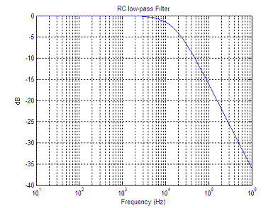
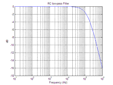
For R1 = 10k and C1 = 1 nF, the obtained result is:  For R1 = 1k and C1 = 1 nF, the obtained result is:  As before, we can now use WinSpice as if it was another built-in Matlab function! This means that we can work through circuit optimization using functions such as 'fminbnd' or 'fminsearch'... We can try some numbers in our design, we can see the results and use Matlab to modify relevant values in the circuit, iteratively... Reference: http://desi.iteso.mx/erayas/cad.htm, 2014. Electronic Experiments Creative Electronics Electrical Calculations From 'Circuit Simulator' to home From 'Circuit Simulator' to Matlab Programming Top |


