Fourier
Series - an understandable introduction...
In
mathematics, the Fourier
series is an infinite sequence
of terms used to solve special types of problems.
The series consists
of an
infinite sum of sines
and cosines that repeats over fixed intervals, and so is
very useful for analyzing periodic functions.
Fourier
theorem is the key to the analysis in the frequency
domain when talking about electronic applications.
According to the Fourier
theorem, a wave or signal is composed of a series of
sinusoidal components
whose frequencies are those of the fundamental freq. and its harmonics, each
component having the proper amplitude and phase. The sequence of
components
that form this wave is called its spectrum.
There are, at least, two ways to perform a circuit analysis.
First, you can find what happens with the periodic waveform at every
instant of
time; second, you can determine what happens to each of its harmonics.
Sometimes, the first analysis (time
domain) is fast, but often the second
analysis (frequency domain)
is better.
Spectral components
Suppose Vp-p
represents
the peak-to-peak value of a sawtooth wave. It can be demonstrated that
the
amplitude of each harmonic is
Vn
= Vp-p /(nπ)
This means that the peak value of the nth
harmonic is equal to Vp-p
divided by nπ.
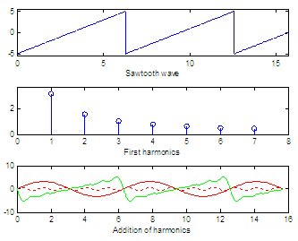
For
example, the top subplot in this figure shows a sawtooth
wave with a peak-to-peak value of 10,

the harmonics have then the following peak
values:
V1
= 10/(1π) = 3.18
V2
= 10/(2π) = 1.59
V3
= 10/(3π) = 1.06
The second subplot in the figure above shows the first seven magnitudes
of the
respective harmonics. The bottom subplot shows how the addition of
different
harmonics (red lines) can produce something close to the original
sawtooth
(green line): the more considered terms the more accuracy.
You can learn some ideas
on how to produce periodic square
or sawtooth waves, here.
The Matlab code to
produce the first two subplots in the
figure above, is:
x = 0 :
.01 : 5*pi;
y = 5 *
sawtooth(x);
subplot(311),
plot(x, y)
axis([min(x)
max(x) min(y)-.5 max(y)+.5])
xlabel('Sawtooth
wave')
n = 1 :
7;
v = 10
./(n*pi);
subplot(312),
stem(n, v)
axis([min(n)-1
max(n)+1 0 max(v)+.5])
xlabel('First
harmonics')
With an oscilloscope (time domain tool) you can see the periodic signal
as a
function of time. The vertical axis represents voltage and the
horizontal axis
represents time, in fact, the oscilloscope represents the instantaneous
value V of the periodic wave.
The spectrum analyzer is different because it’s an instrument of the
frequency
domain. The horizontal axis represents the frequency, and the vertical
axis
represents the amplitude of the harmonics. For example, you would use
an
oscilloscope to observe the top subplot above. You’d use a spectrum
analyzer to
observe the middle subplot above (that's what the Fourier series are
for). This kind of information is called
the
spectrum, where each level of the vertical lines represents the peak
value of
the harmonics, and the horizontal axis shows the corresponding
frequency.
Any periodic wave has a spectrum or a set of vertical lines
representing the
harmonics. The spectrum naturally differs from one periodic signal to
another.
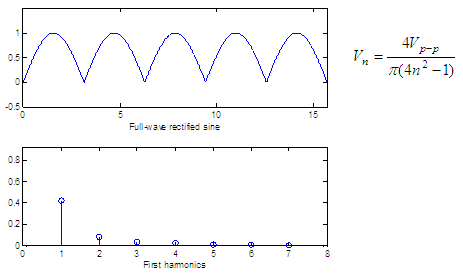
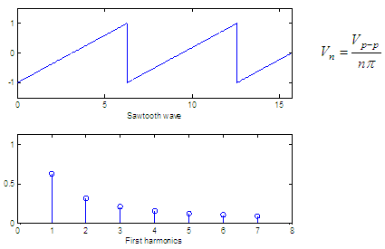
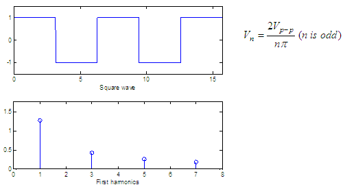
Three basic spectra
The figures below show
three periodic waves and their spectra. In each case, Vp-p
is the peak-to-peak value
of the periodic wave and for convenience we show only the harmonics up
to n = 7. The formula of the
harmonic peak
appears for each case.


You
can learn some ideas on how to produce square and sawtooth functions,
here.
The code to
produce the Fourier series of harmonics above is:
clear,
clc, close all
x = 0 :
.01 : 5*pi;
y =
sawtooth(x);
subplot(211),
plot(x, y)
axis([min(x)
max(x) min(y)-.5 max(y)+.5])
xlabel('Sawtooth
wave')
n = 1 :
7;
v = 2
./(n*pi);
subplot(212),
stem(n, v)
axis([min(n)-1
max(n)+1 0 max(v)+.5])
xlabel('First
harmonics')
figure
y =
square(x);
subplot(211),
plot(x, y)
axis([min(x)
max(x) min(y)-.5 max(y)+.5])
xlabel('Square
wave')
n = 1 :
2 : 7;
v = 4
./(n*pi);
subplot(212),
stem(n, v)
axis([min(n)-1
max(n)+1 0 max(v)+.5])
xlabel('First
harmonics')
figure
y =
abs(sin(x));
subplot(211),
plot(x, y)
axis([min(x)
max(x) min(y)-.5 max(y)+.5])
xlabel('Full-wave
rectified sine')
n = 1 :
7;
v = 4
./(pi*(4*n.^2 - 1));
subplot(212),
stem(n, v)
axis([min(n)-1
max(n)+1 0 max(v)+.5])
xlabel('First
harmonics')
Reference:
Malvino, A. P.; Electronic Principles; 2nd. edition; McGraw-Hill Co.,
1979.
From
' Fourier Series ' to
home
From
' Fourier
Series ' to Calculus Problems


|


