

The Magic Square (an introduction to matrices)In Matlab, a matrix is a rectangular array of numbers. A scalar is a special 1-by-1 matrix, and matrices with only one row or column, are vectors. The operations in Matlab are designed to be as natural as possible. Some programming languages work with numbers one at a time, but Matlab allows you to work with entire matrices easily and quickly.
The best way for you to get started with Matlab is to learn how to handle matrices. You can enter matrices into Matlab in several different ways:
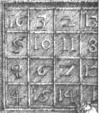
Enter Durer’s matrix as a list of elements. You only have to follow a few conventions:
M = [16 3 2 13; 5 10 11 8; 9 6 7 12; 4 15 14 1] Matlab displays the matrix you just entered. M = 16 3 2 13 5 10 11 8 9 6 7 12 4 15 14 1 This matches the numbers in the picture. Once you have entered the matrix, you can refer to it simply as 'M'. Now that you have M in the workspace, take a look at what makes it so appealing. Is it a magic square? You are probably aware that the special properties of a magic square have to do with the various ways of summing its elements. If you take the sum along any column or row, or along either of the two diagonals, you will always get the same number. Let us verify that using Matlab. The first statement to try is sum(M) Matlab replies with ans = 34 34 34 34 When you do not specify an output variable, Matlab uses the variable ans, to store the results of a calculation. You have found a row vector containing the sums of the columns of M, and each of the columns has the magic sum, 34. How about the row sums? The easiest way to get the row sums is to transpose the matrix, compute the column sums of the transpose, and then transpose the result. The transpose operation is denoted by an apostrophe, '. It flips a matrix about its main diagonal and turns a row vector into a column vector. So, M' produces ans = 16 5 9 4 3 10 6 15 2 11 7 14 13 8 12 1 And sum(M')' produces a column vector containing the row sums ans = 34 34 34 34 The sum of the elements on the main diagonal is obtained with the sum and the diag functions. diag(M) produces ans = 16 10 7 1 and sum(diag(M)) produces ans = 34 You have verified that the matrix in Durer’s engraving is indeed a magic square and have tried a few Matlab matrix operations. The element in row i and column j of M is denoted by M(i,j). For example, M(3,2) is the number in the third row and second column. For our magic square, M(3,2) is 6. So, to compute the sum of the elements in the third column of M, type M(1,3) + M(2,3) + M(3,3) + M(4,3) This produces ans = 34 It is also possible to refer to the elements of a matrix with a single subscript, M(k). This is the common way of referencing row and column vectors. But it can also apply to a fully two-dimensional matrix, in which case the array is regarded as one long column vector formed from the columns of the original matrix. So, for our magic square, M(6) is another way of referring to the value 10 stored in M(2,2). The colon ‘:’ is one of the most important Matlab operators. It occurs in several different forms. The expression 1:8 is a row vector containing the integers from 1 to 8 1 2 3 4 5 6 7 8 To obtain spacing, specify an increment. For example, 100 : -7 : 70 is 100 93 86 79 72 and 0 : pi/10 : pi/2 is 0 0.3142 0.6283 0.9425 1.2566 1.5708 Subscript expressions involving colons refer to sections of a matrix. M(1:k , j) is the first k elements of the jth column of M. So, sum(M(1:4,4)) computes the sum of rows 1 to 4, along column 4. But there's even a better way. The colon by itself refers to all the elements in a row or column of a matrix and the keyword end refers to the last row or column. So, sum(M(:,end)) computes the sum of the elements in the last column of M. ans = 34 Matlab actually has a built-in function that creates magic squares. This function is named 'magic'. So, N = magic(4) displays a 4-by-4 matrix N = 16 2 3 13 5 11 10 8 9 7 6 12 4 14 15 1 This matrix is almost the same as the one in the Durer's picture and has all the same magic properties; the only difference is that the two middle columns are exchanged. Noticed? To make this N into Durer’s M, swap the two middle columns: M = N(: , [1 3 2 4]). This means, for each of the rows of matrix N, reorder the elements in the order 1, 3, 2, 4. It produces M = 16 3 2 13 5 10 11 8 9 6 7 12 4 15 14 1 From 'Magic Square' to home From 'Magic Square' to 'Matlab Help Menu' Credits: Albrecht Dürer, Public domain, via Wikimedia Commons
|

