
Nonlinear Programming (NLP) based on Optimization Techniques
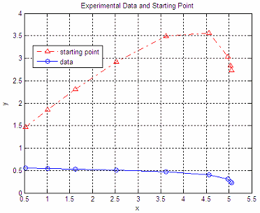
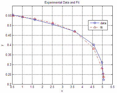
This explanation is neither formal nor comprehensive, but straightforward and useful. Nonlinear programming is a quite broad field, and practical approaches are sometimes required for better understanding. Example. Curve Fitting Let's say that we obtained some data experimentally. We want that information (data) to match a given equation. That's called curve fitting. Let's say that we experimentally obtained these points: data = [0.5243 0.5539 1.0156 0.5436 1.6243 0.5294 2.5266 0.5057 3.6132 0.4698 4.5650 0.4013 4.9739 0.3117 5.0357 0.2536 5.0604 0.2223]; Let the first column of the table be our independent variable (x), and the second column be our dependent variable (y). On the other hand, we want to find out the coefficients for an equation of the form: y = C1 + C2*x + C3*log(1 - z/5.1), that match the above data, where z = 1.0255*x - 0.2722 We can solve this problem using optimization techniques intended for typical nonlinear programming cases. A good built-in function to achieve this is 'fminsearch'. It implements the Nelder-Mead method (simplex direct). 'fminsearch' finds the value of the variables that can produce a minimum point in a given function (your objective function), and it's a standard function, you don't need any special Matlab toolbox. This instruction finds local minima, not global ones. First, we need to define an objective function (OF). We have to express our problem in such a way that its minimum value represents our solution. There are many ways to do this, but its definition certainly impacts the result. We want only a solution to our problem (an engineering approach), not the best solution (a mathematical approach). For our example, we can try this Objective Function:
y2 =
C(1) + C(2)*x + C(3)*log(1 - z/5.1); This m-file will be iteratively called by 'fminsearch'. It modifies the coefficients in C and finds out the value of the function (y2). Then, it subtracts it from y (the original obtained data) and gets the so-called Manhattan norm of the difference. 'fminsearch' uses this returned scalar number to find out the next C values. It goes on and on until it can't improve any more according to a given tolerance that you can define (using 'optimset'). A zero value of this objective function means that y = y2 and that C contains the best possible coefficients. We can call this objective function with a script like this:
data = [ x =
data(:, 1); y = data(:, 2); fx = 'OF_nl_prog'; These are our results: C
= 0.5488
0.0130 0.1128

It works, right? From 'Nonlinear Programming' to home From 'Nonlinear Programming' to 'Matlab Programming'
|

