Random Numbers and Simulations

Averages

There’s a Matlab command which does exactly this: ‘mean(x)’. 

There’s another related command, which is ‘median(x)’ and it’s the value in the ‘middle’ of a vector when the data has been sorted. If there’s an odd number of pieces of data this is well defined, however if the number is even then the mean of the data at each end of the central interval is given, for example the median of [1 2 3 4] is (2+3)/2 = 2.5 whereas the median of [1 3 5] is 3. Note that the median can equal the mean but it is not necessarily so. 

This short code 

x = [4 0 5 3 2 1 3 5 9 3 7 5 6 8 2 0];
mn = mean(x)
md = median(x) 

results in 

mn = 3.9375
md = 3.5000

Other Statistical Measures 

In the previous section we have discussed averages of a set of data but there are more measures available, for instance these two distributions have the same mean but are obviously different in form:

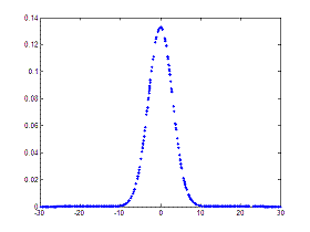
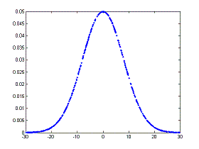
The first curve is narrower than the second and this is quantified using the variance, which is given by

Random Numbers and Distributions

In order to generate random numbers we can use various commands available
in Matlab. We won’t worry about how this is done or the technical aspects of the seeding. We’re going to start with the simple command ‘rand’ which returns a random number between zero and one. 

If we rolled a die a large number of times, and we used the above formulas to calculate the mean and variance, we’d expect to obtain a mean = 3.5 and a variance = 2.916. Let’s try it with Matlab. 

function n = roll_d()
n = ceil(rand*6 + eps);
 

We can use it like this: 

% Roll the die and keep the values in d
for i = 1 : 1000
    d(i) = roll_d;
end 

% Find how many appearences of each possible value
for i = 1 : 6
    v(i) = length(find(d==i));
end 

% Display results
disp(['Mean = ' num2str(mean(d))])
disp(['Variance = ' num2str(var(d))])
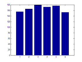
bar(v) 

The results are: 

Mean = 3.508
Variance = 2.7827

Obviously, every time that we run the program we’ll get different results, since we are dealing with random numbers, but the results are similar to what we expected.

We can use this process for other ‘chance games’, for example tossing a coin: 

function r = toss()
p = ['heads'; 'tails'];
i = ceil(rand*2 + eps);
r = p(i,:); 

This can then be called just using 'toss' which generates either 'heads' or 'tails'.

Normal Distribution 

A normal distribution has two parameters associated with it: the mean and the variance. The command ‘randn’ generates random numbers which have a mean of zero and a variance of unity. 

By typing 

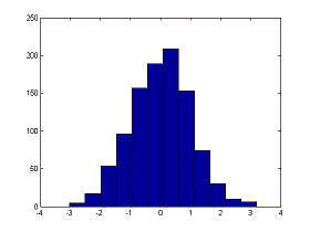
x = randn(1, 1000);
hist(x,12) 

we set up an array and produce the plot

These lines on the command window 

mn = mean(x)
v = var(x) 

produce, in our case 

mn = 0.0016
v = 0.9908 

which are values very close to what was expected.

There are many problems which require simulation, largely due to that it's not viable to actually run the real or physical tests. These cases cover things from experiments on aircrafts or cars (which are too dangerous or expensive) to population studies and economic strategies.