Scilab 3D PlotsIn this brief article we’re going to describe how to create 3D Plots in Scilab. We can use built-in functions very similar to Matlab’s, such as meshgrid, plot3d, surf and others... or we can use a more native function such as param3d (as always, you can type ‘help’ on your Scilab command window to see a comprehensive list of available functions).It is necessary to have
three vectors containing x, y and z
values of the coordinates that we want to display. This is the syntax param3d(x, y, z, [theta, alpha, leg, flag,
ebox]) where - x, y and z are three vectors of the same size representing points of the parametric curve. - theta and alpha are real values containing the spherical coordinates of the observation point (in degrees). - leg is a string defining the labels for each axis with @ as a field separator, for example "X@Y@Z". - flag = [type, box]; type and box have the same meaning as in plot3d: type is an integer used for scaling, and box is an integer to describe features of the frame around the plot. - ebox specifies
the boundaries of the plot as the vector [xmin,
xMax, ymin, yMax, zmin, zMax]
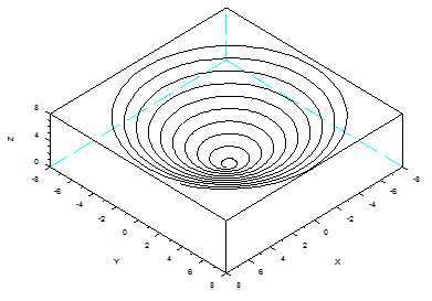
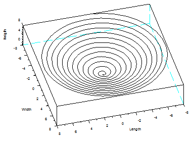
z = 0 : .01 : 8; scf();
At the top of figure
windows you can find the Tool option
and then the 2D/3D Rotation option. This can help you visualize the
plot from
different angles. Other functions for 3D Plots in Scilab
meshgrid - create
matrices or 3-D arrays Examples
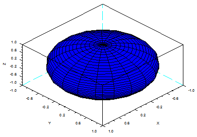
// Generate a sphere,
default view
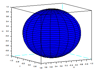
// the same shape but other
values for theta and alpha
angles
From 'Scilab 3D Plot' to Matlab home From 'Scilab 3D Plot' to Scilab Menu
|