Nonlinear Simultaneous Equations

 
We’re going to develop a Matlab function to solve systems of nonlinear simultaneous equations. We’ll use the ‘fminsearch’ function to find the intersection of the given curves or functions with several variables. The method ends when a solution is found, when a maximum number of iterations is reached, or when some specifications of tolerances are met, according to the default options for fminsearch.    

For each system of nonlinear equations and starting points, we need to be aware of the solution found, the number of iterations needed, the number of function evaluations needed, and the exit flag value. This helps us know whether the found solution is good or bad.  

It’s important to note that this minimization or optimization function (fminsearch) doesn’t solve simultaneous equations. We have to adapt the system or formulate the problem in such a way that we can accomplish this. In this particular case, we’re going to express the nonlinear system as a scalar value, and it’s going to be reduced to its minimum value by fminsearch. That value will be the solution to our problem.  

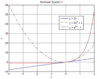
Naturally, different tolerances or starting points deliver different results. Only one intersection is found for every starting point, even though the nonlinear system may have more than one solution.  

If we have this nonlinear system of simultaneous equations:

 
We can express the system in Matlab as a function returning a scalar:

function y = nls1(x)
y1 = 2 * x;
y2 = 4* x^2 + x;
y3 = exp(2 * x) - 1;
y = norm(y1-y2-y3, 2);
 

We expect y to be zero at the end (where the curves intersect). If not, the solution is not good enough. fminsearch will find the value of x that minimizes the expression |y1 - y2 - y3|. Of course, we can formulate or express the system in different ways. This is only one idea and this function is called the ‘objective function’, in numerical optimization terms.  

Finally, we can minimize this type of systems with an optimization instruction ('fminbnd' for one variable or 'fminsearch' for one or more variables). We provide two parameters, both the name of the nonlinear system and the starting point (we’re using the default options, which can be modified with ‘optimset’).  

fx = 'nls1';
x0 = -5
[x_sol, f, EF, out] = fminsearch(fx, x0)
 

The answer is: 

x_sol = 0
f = 0
EF = 1
out =
    iterations: 20
     funcCount: 41
     algorithm: 'Nelder-Mead simplex direct search'  
 

Now, we can try a different starting point, to compare solutions: 

x0 = 10
[x_sol, f, EF, out] = fminsearch(fx, x0)
 

The new answer is: 

x_sol = 0
f = 0
EF = 1
out =
    iterations: 21
     funcCount: 43
     algorithm: 'Nelder-Mead simplex direct search'      
 

Note that the solution in both cases is almost the same (within the default tolerance), but the number of function evaluations is not the same.
 

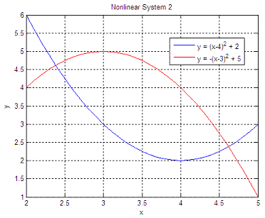
Another example. Let’s solve this system:

 
Our ‘objective function’ is defined:
 

function y = nls3(x)
y1 = (x - 4)^2 + 2;
y2 = -(x - 3)^2 + 5;
y = norm(y1-y2, 2);
 

We run the script like this:

 
fx = 'nls3';
x0 = -20
[x_sol, f, EF, out] = fminsearch(fx, x0) 

x0 = 15
[x_sol, f, EF, out] = fminsearch(fx, x0) 

The two solutions are:
 

x0 = -20
x_sol = 2.3820
f = 3.5793e-005
EF = 1
out =
    iterations: 23
     funcCount: 47
    

x0 = 15
x_sol = 4.6180
f = 1.0069e-004
EF = 1
out =
    iterations: 21
    funcCount: 43

We find both solutions, x1 = 2.382 when we start at x0 = -20, and x2 = 4.618 when we start at x0 = 15.

From 'Nonlinear Simultaneous Equations' to home
From 'Nonlinear Simultaneous Equations' to Matlab Programming