Solid of Revolution – Cylinders in Matlab

Revolving a 2D function about the x-axis

Naturally, you can always type 'help cylinder' on your command window to see the explanation and examples of this function.

The basic format [X, Y, Z] = cylinder(r) returns the x, y, and z-coordinates of a cylinder using r to define a profile curve. cylinder treats its first argument as a profile curve. It’s important to note that the resulting surface object is generated by rotating the curve about the x-axis, and then aligning it with the z-axis.  

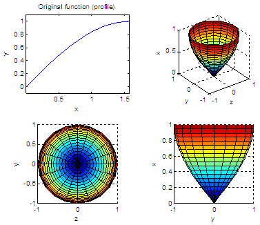
Let’s say that we want to plot a section of the trigonometric sine function, from 0 to П/2, and then rotate it about the x-axis. We can do this:
 

% Clear memory, clean screen, close any figure
clear, clc, close all 

% Define our initial profile
x = linspace(0, pi/2, 20);
y = sin(x); 

% We draw the profile
subplot(221), plot(x,y), axis equal
title('Original function (profile)')
xlabel('x'); ylabel('y'); 

% We use the cylinder function to rotate and align
% with the z-axis, to produce a 3D solid
[X,Y,Z] = cylinder(y);
subplot(222), surf(X,Y,Z), axis square
xlabel('z'); ylabel('y'); zlabel('x') 

% We can have another view, along the x-axis
subplot(223), surf(X,Y,Z), axis square
xlabel('z'); ylabel('y'); zlabel('x')
view(0,90)

% We produce another image, now a lateral view
subplot(224), surf(X,Y,Z), axis square
xlabel('z'); ylabel('y'); zlabel('x')
view(90,0)
 

Let’s note that the shape or envelop is what we want. When we rotate the line, the x-limits are lost, and and become 0 to 1. We keep the idea for this 3D image, though.

If we interchange the parameters for the surf function, we can achieve another views. We can play with coordinates and labels. Keep an eye on the axes, values and labels, so you can know what you’re seeing.

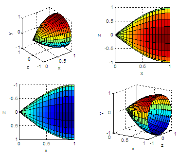
% Let's create another figure and plot it from the back
figure
subplot(221), surf(Z,X,Y), axis square
xlabel('x'); ylabel('z'); zlabel('y') 

% A view from the top, showing high y-values
subplot(222), surf(Z,X,Y), axis square
xlabel('x'); ylabel('z'); zlabel('y')
view(0,90) 

% A view from the bottom, showing low y-values
subplot(223), surf(Z,X,Y), axis square
xlabel('x'); ylabel('z'); zlabel('y')
view(0,-90) 

% A final arbitrary view for this solid of revolution
subplot(224), surf(Z,X,Y), axis square
xlabel('x'); ylabel('z'); zlabel('y')
view(35, 15)

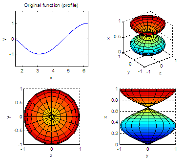
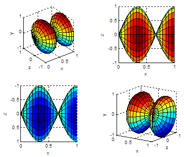
Let’s change the limits and profile function (first lines above), keep the rest of the code as it is, and see the interesting solids of revolution and pretty images that we get:
 

x = linspace(pi/2, 2*pi, 20);
y = cos(x);