Taylor expansion - series experiments with MatlabOnce you know how Maclaurin series work, Taylor series are easier to understand.Taylor expansions are very similar to Maclaurin expansions because Maclaurin series actually are Taylor series centered at x = 0. Thus, a Taylor series is a more generic form of the Maclaurin series, and it can be centered at any x-value. The goal of a Taylor expansion is to approximate function values. You’ll have a good
approximation only if you’re close to the series’
center.
Note: Other
than that, the formulas (Maclaurin’s and Taylor’s) are identical.
And we’ll need to take
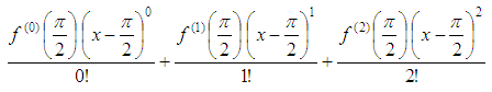
three derivatives (n = 0 to 2) of
the function and then
evaluate them at x = pi/2. Definition 1: f(0)(x)
is the function itself, in this case
cos(x). It's not a derivative! f(0)(x)
= cos(x)
f(0)(pi/2) = cos(pi/2)
= 0
clear,
clc %
Let's see more decimals %
We go from n = 0 to n = 2 %
Center and point to evaluate %
These are the derivatives for each term %
We form the sequence, following the Taylor formula %
We add-up to get the Taylor approximation %
Let's compare with the official number
seq =
0 -0.02920367320510
0 We’ve got almost the
exact value by using only 3 terms of
the series (and two
values are zero because the derivative is zero for
those
terms!!). If we had used n = 10, it
would have been an even better approximation. Now, let’s develop an automated series to express the cosine function (centered at pi/2) using the Taylor expansion and let’s compare the results with different number of terms included. function stp =
taylor_cosine(c, x, n) %
Start the series with 0 %
Consider all the possible derivatives %
Iterate n times (from 0 to n-1)
% Implement the Taylor
expansion
% Find derivative for the next
term end %
Add-up the calculated terms Note:
the above code is not very efficient, because we’re calculating and
adding
terms even when their derivative is zero, which is a waste of 50% of
the time,
more or less. We’ll leave it as-is just to keep and show the natural
flow of
the formula... Now,
let’s create a script to test and use the function above. clear,
clc, close all %
Work with values around center c %
Plot the goal %
Consider 4 terms in the series %
Consider 6 terms %
Consider 10 terms %
Label the calculated lines
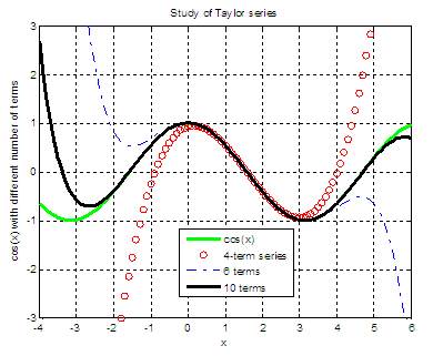
We see that all of the
Taylor expansions work well when we
are close to pi/2 (x approx. 1.57). More terms approximate better a
larger
portion of the cosine curve. Maclaurin Series Sequences Fourier Analysis - intro Fourier Series From 'Taylor Expansion ' to home From 'Taylor Expansion ' to Calculus Problems Top
|