

3D Plot – Part 1
From '3D Plot Part 1' to 3D Main
Matlab provides many powerful instructions for the visualization of 3D data. The instructions provided include tools to plot wire-frame objects, 3D plots, curves, surfaces... ... and can automatically generate contours, display volumetric data, interpolate shading colors and even display non-Matlab made images. Here are some commonly used functions (there are many more):
Among these instructions, plot3 and comet3 are the 3D matches of plot and comet commands mentioned in the 2D plot section. The general syntax for the plot3 command is plot3(x, y, z, 'style') This command draws a 3D curve with the specified line style. The argument list can be repeated to make overlay plots, just the same way as with the plot command in 2D. We have to make some necessary comments before any example can be introduced. Plots in 3D may be annotated with instructions already mentioned for 2D plots: xlabel, ylabel, title, legend, grid, etc., plus the addition of zlabel. The grid command in 3D makes the appearance of the plots better, especially for curves in space. View The viewing angle of the observer is specified by the command view(azimuth, elevation), where
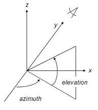
By specifying appropriate values of azimuth and elevation, one can plot projections of 3D objects on different 2D planes. For example, the command ' view(90,0)' places the viewer toward the positive x-axis, looking straigth on the yz-plane, and thus produces a 2D projection of the object on the yz-plane. ' view(0, 90)' shows the figure on a 2D xy-plane. The following script generates data, plots the curves and obtains different views. Example: % clears variables, command window and closes all previous figures clear; clc; close all % generates an angle vector with 101 values a = 0: 3*pi/100 : 3*pi; % calculates x, y, and z x = cos(a); y = sin(a); z = a; % divides the figure window into 4 subwindows (2x2) % plots on the 1st. one subplot(2,2,1) plot3(x,y,z) grid on title('A helix - 3D view') xlabel('x = cos(a)') ylabel('y = sin(a)') zlabel('z = a') % plots on the 2nd. subwindow subplot(2,2,2) plot3(x,y,z) axis('square') % rotates the figure to show only the xy-plane view(0,90) grid on title('A helix, xy-plane') xlabel('x = cos(a)') ylabel('y = sin(a)') zlabel('z = a') % plots on the 3rd. subwindow subplot(2,2,3) plot3(x,y,z) % rotates the figure to show only the xz-plane view(0,0) grid on title('A helix, xz-plane') xlabel('x = cos(a)') ylabel('y = sin(a)') zlabel('z = a') % plots on the 4th. subwindow subplot(2,2,4) plot3(x,y,z) % rotates the figure to show only the yz-plane view(-90,0) grid onundefined title('A helix, yz-plane')undefined xlabel('x = cos(a)')undefined ylabel('y = sin(a)')undefined zlabel('z = a')undefined undefined undefined undefined And the result is:undefined undefined undefined
undefined
undefined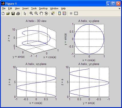 undefined undefinedundefined undefinedundefinedMatlab-Examples homeundefined undefined undefinedFrom '3D Plot Part 1' to 3D Main Menuundefined undefined undefined undefined undefined undefined undefined undefined undefined undefined
undefined undefined undefined undefined undefined undefined
undefined |
undefined undefined undefined undefined undefined undefined undefined undefined undefined undefined undefined |
 undefined
 undefined