
3D plot – Part 2Modeling Surfaces, Meshes and 3D variationsThe 3D plot functions intended for plotting meshes and surfaces ' mesh' and ' surf', and their several variants ' meshc', ' meshz', ' surfc', and ' surfl', take multiple optional input arguments, the most simple form being ' mesh(z)' or ' surf(z)', where z represents a matrix.
Meshgrid Suppose that you want to plot the function z = x 2 – 10y + 2 over the domain 0 ≤ x ≤ 4 and 0 ≤ y ≤ 4. To do so, we first take several points in the domain, say 25 points, as shown in this Fig.: 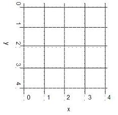
We can create two matrices x and y, each of size 5 x 5, and write the xy-coordinates of each point in these matrices. We can then evaluate z with the command z = x.^2 – 10*y + 2. However, creating the two matrices x and y is much easier with the meshgrid command. % creates vectors x and y, from 0 to 4 vx = 0 : 4 vy = vx % creates meshgrid to be used in 3D plot [x,y] = meshgrid(vx,vy) The commands shown above generate the 25 points shown in the figure. All we need to do is generate two vectors, vx and vy, to define the region of interest and distribution or density of our grid points. Also, the two vectors need not be either same sized or linearly spaced. It is very important to understand the use of meshgrid. Matlab response is as follows: vx = 0 1 2 3 4 vy = 0 1 2 3 4 x = 0 1 2 3 4 0 1 2 3 4 0 1 2 3 4 0 1 2 3 4 0 1 2 3 4 y = 0 0 0 0 0 1 1 1 1 1 2 2 2 2 2 3 3 3 3 3 4 4 4 4 4
The folowing script could be an example of how tho use the ' meshgrid', ' plot3', ' meshc', and ' surfc' commands. We'll 3D plot the following surface: 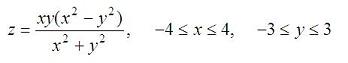
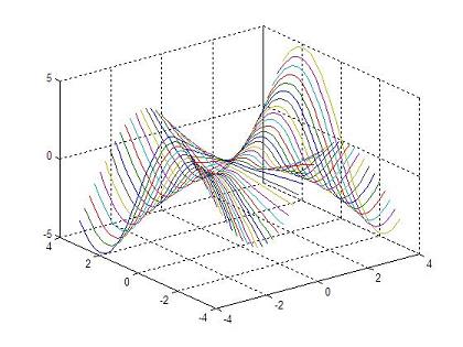
with this script: % clears command window, clears variables and closes figures clc; clear; close all % defines vectors x and y vx = -4 : 0.2: 4; vy = -3 : 0.2: 3; % calculates the necessary grid [x,y] = meshgrid(vx, vy); % calculates z and avoids a null denominator adding 'eps' % (eps is the least possible number in Matlab) z = x .* y .* (x.^2 - y.^2) ./ (x.^2 + y.^2 + eps); % generates the first figure using 'plot3' figure plot3(x,y,z) grid on undefined undefined% generates the second figure using 'meshc' to include theundefined undefined% contour in the figure, and rotates the figure with 'view'undefined figureundefined meshc(x,y,z)undefined view(-37, 15)undefined undefined undefined% generates the third 3D figure using 'surfc' to include theundefined undefined% contour in the image, and also rotates the figure with 'view'undefined figureundefined surfc(x,y,z)undefined view(-47, 25)undefined undefined undefined undefined And the generated results are:undefined undefined undefined undefined
undefined
undefined
 undefined undefinedundefined
undefined
undefined undefined undefinedundefined undefined
undefined
undefined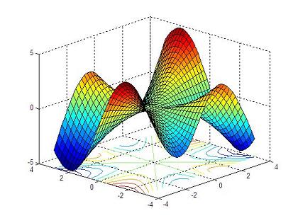 undefined undefinedundefined Do you like it?undefined undefined Use the instruction 'undefinedrotate3d on' to manipulate the view angle of your plot. Include it in your script or type it in the command window to change the view with your mouse over the figure...undefined undefined undefinedFrom '3D Plot part 2' to homeundefined undefined undefinedFrom '3D Plot part 2' to 3D Mainundefined undefined undefined
undefined undefined undefined undefined undefined undefined
undefined |
undefined
undefined undefined undefined undefined undefined undefined undefined undefined undefined undefined undefined undefined undefined undefined undefined undefined undefined undefined undefined undefined undefined undefined undefined undefined undefined undefined undefined undefined undefined undefined undefined undefined undefined undefined undefined |
undefined
 undefined