Mathematical Optimization using Scilab

In Scilab, we can perform mathematical optimizations using the built-in function named ‘optim’. We need to define the function to be optimized, with some special pecularities to take into account. Our function not only takes its regular arguments, but there’s also a parameter indicating what it is expected to deliver. The function must output its value and maybe its gradient and an index to notify special cases. 

So optim is another non-linear optimization routine and it’s based on derivatives. We have seen polynomial fitting and least squares-based algorithms in other examples. 

In general, the form of the function to be minimized or optimized is:

[fx, gr, ind2] = f(x, ind1, p1, p2, ...) 

where
ind1 = 2 means that we’re evaluating fx = f(x).
ind1 = 3 means that we’re evaluating gr = f’(x).
ind1 = 4 means that we’re evaluating both the function and its gradient.
ind2 < 0 notifies that the function was not able to evaluate f(x).
ind2 = 0 means that the optimization didn’t finish correctly.
p1, p2, ... are aditional parameters that the function could take 
 

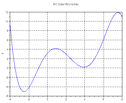
We are going to see a simple example where we want to minimize a 5th. order polynomial.
 

This is our polynomial:

y = -0.0071x⁵ + 0.087x⁴ - 0.1x³ - 1.3x² + 2.3x + 3.2

 
and this is the correspondig plot: 

x = -4 : .01 : 8;
y = -.0071*x^5 + .087*x^4 - .1*x^3 - 1.3*x^2 + 2.3*x + 3.2;
plot(x, y)
xgrid
title('5ht. Order Polynomial'); xlabel('x'); ylabel('y')

This is the code that we could use to find its minimum value: 

// We define the function
function f = poly5(x)
  f = -.0071*x^5 + .087*x^4 - .1*x^3 -1.3*x^2 + 2.3*x + 3.2;
endfunction 

// We define the objective or cost function. We need to
// calculate the gradient. In this case we're using the
// built-in function numdiff to calculate it
function [f, g, ind] = poly5Cost(x, ind)
  if ((ind == 1) | (ind == 4))
    f = poly5(x);
    g = numdiff(poly5, x);
  end
endfunction 

// We have to make an initial guess
x0 = 0; 

// Now we use the optim function which calls the
// previously defined objective function
[yopt, xopt] = optim(poly5Cost, x0)
 

The result of our mathematical optimization according to Scilab is: 

xopt  = -2.5130895
yopt  = -5.021364
 

Notice that this result is a local minimum. Actually, the function minimum is a number that tends toward minus infinity (not plotted). 

If we start with another seed, we can get a different result, for example 

x0 = 8;
[yopt, xopt] = optim(poly5Cost, x0) 

produces:
xopt  = 4.477D+61
yopt  = -1.276+306 

We also can include lower and upper bounds on x, as in 

x0 = 1;
[yopt, xopt] = optim(poly5Cost, 'b', 1, 7, x0) 

which now produces another local minimum
xopt  = 3.8891255
yopt  = 0.1859703
 

A note about the gradient that we need to include as output: we used ‘numdiff’, which is a numerical gradient estimation, and we can also use 
‘derivative’, which approximate derivatives of a function. If you know the exact derivative, you should use it, but it's also possible to optimize a problem without an explicit knowledge of the derivative of the objective function, and the numdiff or derivative function can accomplish this task.