Sine series - working without the sine (or cosine) functionFour ways to code a sine/cosine series in Matlab
Sometimes we just can’t use a trigonometric
function
and we must use an alternative method to generate a table of values,
for
example.
Experiment
1. Let’s code the cosine series to avoid using the cos(x) function
In this case the formula under study is the cosine series, defined as 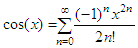
function y =
cos1(x) We’re
not using for-loops (that’s vectorization), but we’re using some
built-in
functions such as sum and factorial. We’re
assumming that x
is a scalar number, and our calculation includes only
100
terms. We’re just implementing the formula above... We must keep in
mind
that
this is an approximation only. If we
test the code by comparing what the actual ‘cos’ function calculates
against
our result, then x = 10; x = 40; We get
from Matlab... ans
= -0.8391 ans
= -0.6669 We can
see that our result is good enough for the first case, but it’s not
good for
the second case. We must take into account that the built-in factorial
function
uses an algorithm with double precision numbers, and since double
precision numbers
only have about 15 digits, the answer is only accurate for N <=
21. We must
be very aware of the limitations of our resources... Experiment
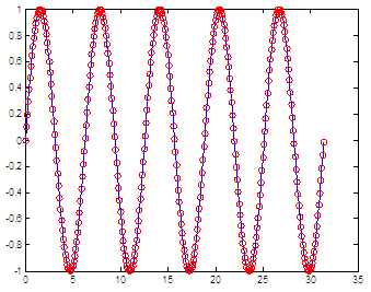
2. We’ll implement the sine series accepting a whole vector now
We’re
going to produce a whole response now, not only a scalar. This function
will
receive a vector and will output another one. The sine series formula
that
we’re going to implement is
Our
proposed code in this case is the following function y =
sin2(x) We are just coding the
formula... We calculate the three parts
of the vectors: the alternating sign (s), the part that contains xi (within the
loop), and the
factorial part (f). Finally
we multiply, divide and sum to produce every response corresponding to
each
element in the input vector. We have to iterate along all of the
elements of
the input vector to obtain all of the elements of the output vector.
Again,
we’re using n = 100, which seems to be a good enough number for our
experiments... We can fastly test the
code, like this x = 0 :
.1 : 10*pi;
Experiment
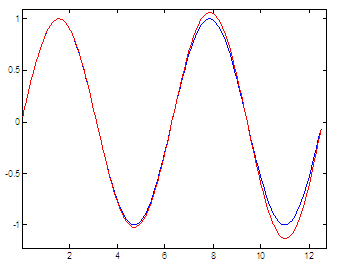
3. We’ll use a product instead of a sum to generate the sine wave
We’re going to implement another formula, shown here
If we use n = 1000, we
can implement an approach of the
series in this way function y =
sin3(x) and a
fast test is achieved in this way x = 0 :
.1 : 4*pi;
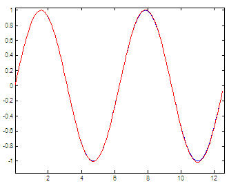
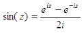
The blue line is the ordinary sine function; the red line is our approximation. We can see that the higher the x-value (angle) the higher number of n elements we have to have in order to obtain a good approximation. It’s all about accuracy in our response. It can deteriorate very easily... Experiment 4. We’ll use exponential functions to generate the sine waveThe definition of the sine function can be extended to complex arguments z, using the definition Another available formula is
This
formula is very easy to evaluate if we have access to exponential
functions and
complex (imaginary) numbers. e is
the
base of the natural logarithm and i
is the imaginary number. The
suggested code is very straightforward function y =
sin4(z)
x = 0 :
.1 : 20*pi; and our
Matlab result is 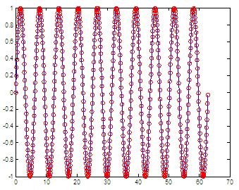
From 'Sine Series' to Matlab Examples home From 'Sine Series' to 'Calculus Problems'
|